Click to Print Adobe PDF 

It seems only yesterday that data storage in radiology was revolutionized by digitization.^1,2 Gone forever are the fat film jackets. No more lost films. If you don’t believe that this was a quantum leap, when was the last time you saw a chest x-ray on a piece of film?

The question everybody keeps asking is why Pathology hasn’t made the same leap. My answer is always the same: we will, but it will take longer, because the digital memory requirements are orders of magnitude greater. One glass slide requires approximately 4 GB of storage. Our laboratory produces approximately 1000 slides per day. Hence, complete digital conversion of our pathology laboratory would require approximately 4 TB (terabytes) of storage per day.

Such memory storage is clearly not currently possible. However, the explosive growth in digital storage capacity of the last several years and the accompanying free-fall in cost are currently accelerating, with no end in sight. As these trends continue, within the next few years, it will be possible, for the first time in human history, to fully digitize anatomic pathology.

Two years ago I predicted that within 10 years, the most advanced Pathology practices across the globe would convert to digital storage and data manipulation, similar to the transformation in Radiology of the past decade. With just eight years left to go, I stand by my original prediction.

This is not say that such a system will be widespread throughout community hospitals, but that it will be spreading, at least on a trial basis, in academic centers and other leading medical institutions.

It is, therefore, appropriate at this time, to explore some of the implications of Pathology’s digital transformation.

APPLICATIONS OF DIGITAL PATHOLOGY

The three main applications of Digital Pathology are telepathology, data storage, and digital-assisted analysis.

Telepathology is currently the most publicized application as it will undoubtedly be indispensible in rural and remote settings where physical travel is arduous and the distances involved are occasionally unreasonable. The reason is obvious and it is easy to understand why telepathology is a popular topic both in the pathology literature and at national meetings. This concept should not be dismissed as a passing fad, but rather recognition of its potential benefit, particular in remote and underserved areas.

Data storage is another well known advantage of digital conversion. In this paradigm, archival glass microscope slides would be to scanned and the data stored digitally. This is no small advantage, since retaining large numbers of glass slides for many years requires not only vast amounts of physical space, but countless person-hours of filing, tracking, retrieval, etc. Regulatory requirements that most slides be retained for a minimum of 20 years force most laboratories, ours included, to rent large amounts of off-site storage space at considerable expense. Furthermore, lost, broken, or misfiled slide may be irreplaceable.

Digital storage also eliminates the need to file and retrieve glass slides. Currently glass slides must be retrieved from the files for tumor boards, for quality assurance, and for comparing current pathology with previous specimens. A busy pathology laboratory can require more than one full FTE dedicated to slide filing and retrieval. As digital storage becomes cheaper, we will reach the point where digital storage is not only easier and more reliable, but also less expensive than maintaining files of glass slides.

Digital mathematical analysis is the most powerful application of digital pathology, yet is, ironically, the least talked about. Probably the two most powerful diagnostic enhancements of digital microscopy are pattern recognition and transformational analysis. The power behind both of these tools is the synergy of the human brain and the computer complementing each other. Some patterns, e.g. certain complex mathematic relationships, are much easier for computers to recognize; other patterns, e.g. facial and voice recognition, seem hard wired into human brains. The computer can easily perform the mathematical transformations that convert data into patterns that our brains immediately recognize.

This is not so esoteric as it sounds. Anyone who has used Photoshop is already framiliar with the advantages of this interaction: it is not that the computer creates something that wasn’t there before. Rather, the computer simply uses a mathematical transformation (digital transformation) to enhance our ability to recognize what was already there. Digital transformation allows us to see what is hidden in plain sight.

MATHEMATICS OF ANATOMIC PATHOLOGY (see Appendix for explanation of terms)

All microscopic analysis is based upon the algebraic relationship between a particular dependent variable and anatomic location in 2-dimensional space. There are innumerable dependent variables which can be analyzed;, the most common are pH, concentration of specific chemical moieties, concentration of specific antigenic epitopes, and number of specific nucleic acid sequences. The independent variable is anatomic location. Each anatomic location occupies a unique position in 2-D space corresponding to a unique 2-dimensional complex number x + iy.

The various relationships between the dependent variables and location are expressed by equations such as:
pH = f(anatomic position)
concentration of antigenic epitope = f(anatomic position) etc.

The may be represented by the equations
pH = f(x + iy)
[Antigen] = f(x + iy)
[Chemical moiety] = f(x + iy)
Etc.

Each microscopic image is a unique pictoral (geometric) solution to one of these equations. Digitization uses analytic geometry to convert this geometric solution to an algebraic solution. The data can then be stored and/or manipulated in digital form.

ALL MICROSCOPIC ANALYSIS IS FUNDAMENTALLY APPLIED ANALYTIC GEOMETRY.

Almost all microscopy involves differential staining of microscopic slides. In other words, the staining intensity varies with some physicochemical parameter, such as pH, electrical charge, antigenic expression, chemical moiety, etc.

Furthermore, this differential staining occurs in situ. In other words, the original anatomic relationships are preserved. This allows, at a microscopic level, mapping of differential physicochemical attributes as a function of anatomic position.

EXAMPLES:

Fig. 1: Eosin Stain: Nucleus pulposus.

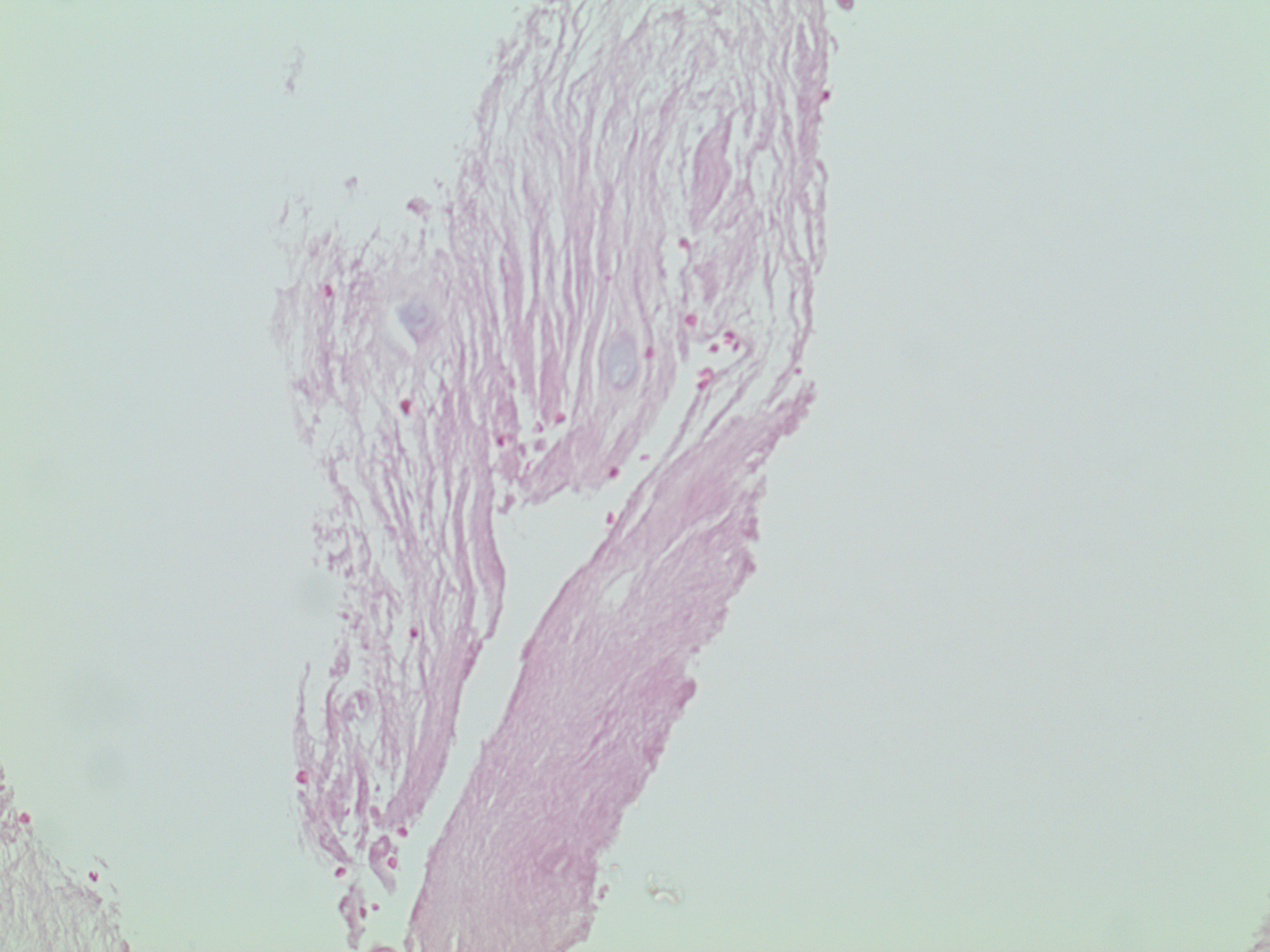
Eosin is a red dye that preferentially binds to acidic (low pH) structures. Note that the original anatomic relationships are retained; hence, this is an in situ stain.
pH = f(anatomic location)
pH = f(x + iy)

Fig. 2: Hematoxylin Stain: H. pylori gastritis.

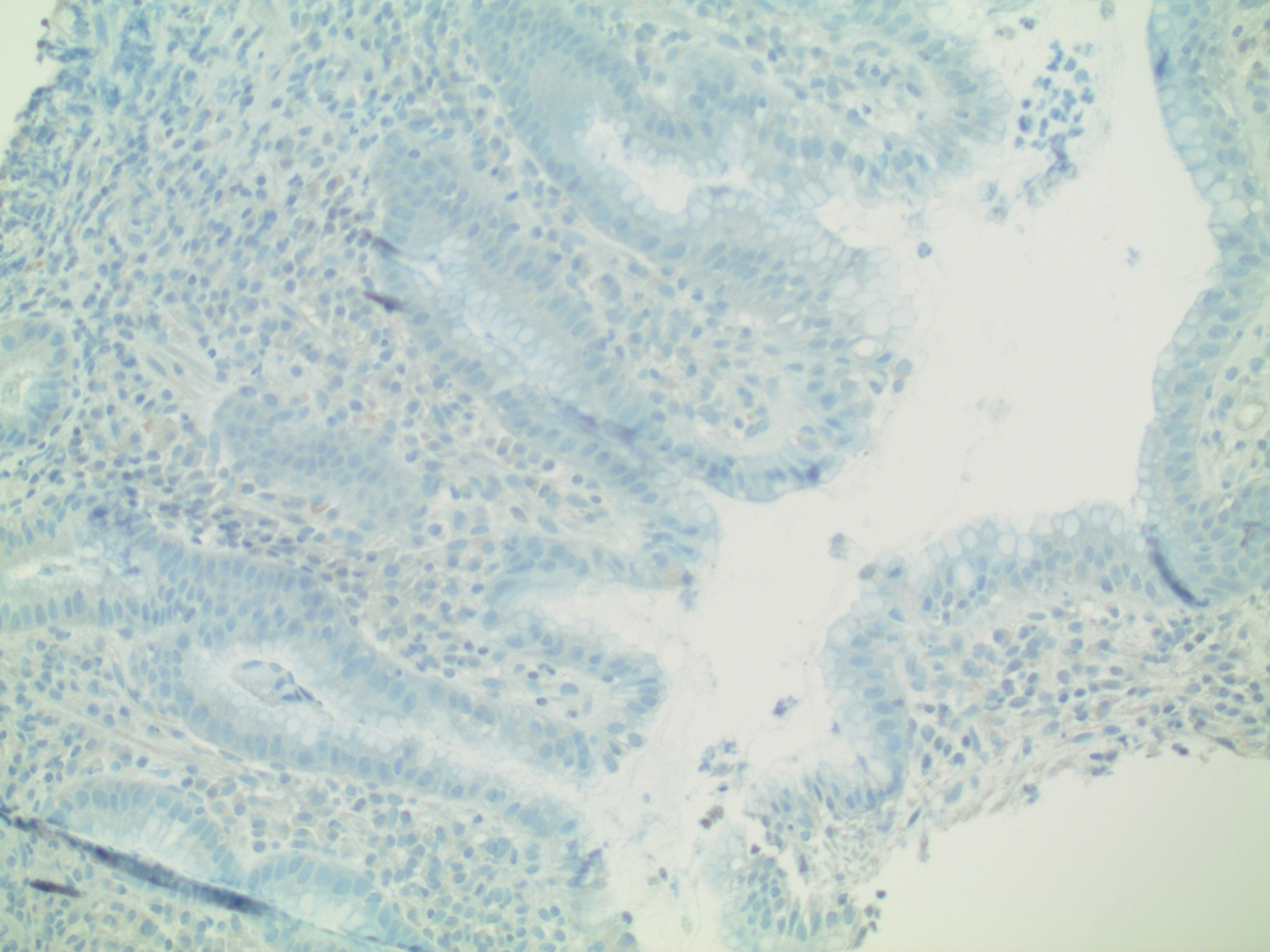
Hematoxylin is a blue due that preferentially binds to basic (high pH) structures. This, too, is an in situ stain. This results in a map showing the relationship between pH and anatomic location. The location of every point in this photograph corresponds to a location in anatomic space, while the darkness (intensity of staining) reveals the pH at that particular point.
pH = f(anatomic location)
pH = f(x + iy)

Fig. 3: Hematoxylin-and-eosin (“H and E”) stain: H. pylori gastritis (same biopsy as Figure 2)

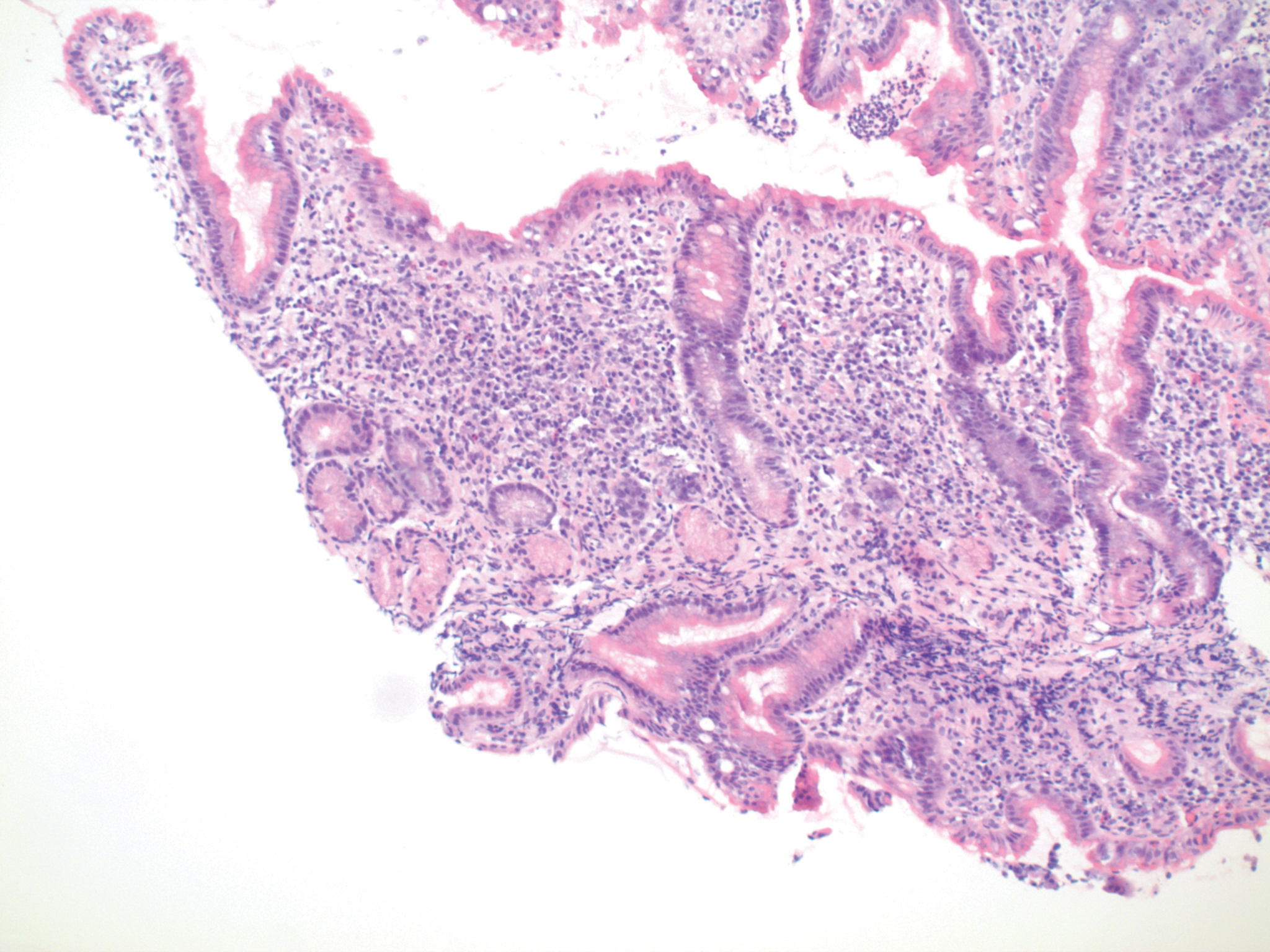
If the same slide is stained with both hematoxylin and eosin, the result is 2-colored in situ staining, with both dyes differentiating by pH. Since each of the two dyes has different optimal binding pHs, the effect is to enhance the mapping of pH as a function of anatomic location.
pH = f(anatomic location)
pH = f(x + iy)

A number of other common stains, including Papanicolaou and Wright stains, are also 2-color in situ differential stains for pH
pH = f(anatomic location)
pH = f(x + iy)

Fig. 4: Two interrelated dependent variables: Immunohistochemical Stain: H. pylori gastritis (same biopsy as Figures 2 & 3)

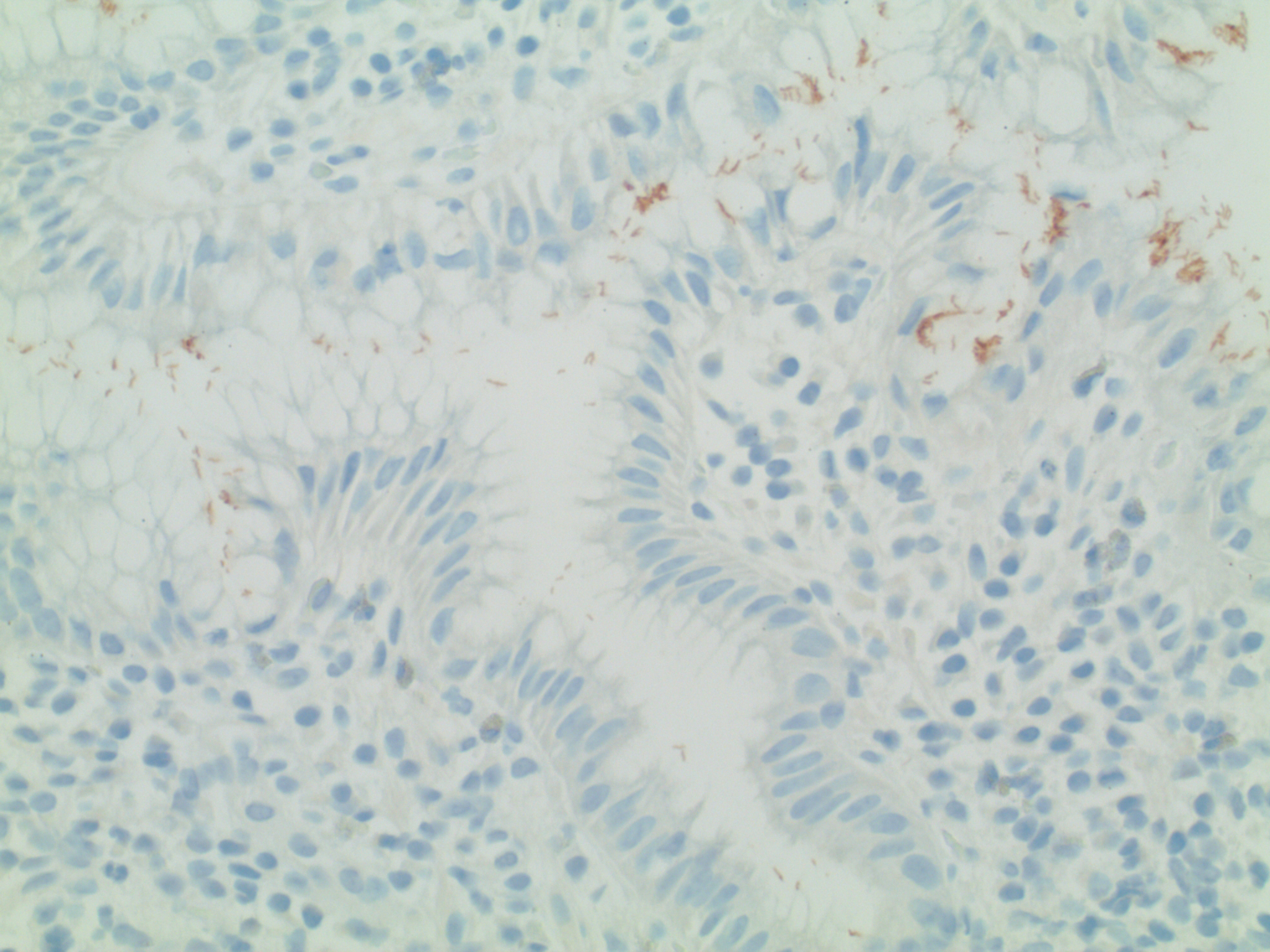
The simplest immunohistochemical stain uses two dyes. The first is a chromagen (usually either red or brown) conjugated to a specific monoclonal antibody. The result is in situ differential staining based upon concentration of the target antigen [Ag].

The second dye is the “background stain”. Its purpose is simply to enhance visibility of the underlying anatomy. The most common background stain is hematoxylin (which, as noted, measures Ph).

In this case, the brown chromagen is conjugated to a monoclonal antibody recognizing Helicobacter pylori. Note that there are three variables, allowing for simultaneous exploration of several relationships, including:
pH = f(anatomic location)
[Ag] = f’(anatomic location)
[Ag] = f”(pH).

This demonstrates the following three mathematic relationships:

• Bacterial antigen expression as a function of anatomic location
• pH as a function of anatomic location
• Bacterial antigen expression as a function of pH

The solution to these three relationships is: Bacteria (brown stain) readily visible in the gastric lumen.

PREPARING FOR THE FUTURE: Quaternion and Vector Analysis in Immunohistochemistry (IHC)

Each location on the microscope slide (or each pixel on the computer) corresponds to a point with multiple “dimensions.” In addition to the conventional two dimensions that describe anatomic location, there are other possible “dimensions” such as pH, and there is no theoretical limit to the number of dimensions each point can represent. For the sake of simplicity let us limit our example to a simple 4-dimensional IHC stain, such as H. pylori detection.

Each point on a simple single antigen immunohistochemical stains has four dimensions, as follows:

• Anatomic location = 2 dimensions (x,y)
• pH / electrical charge = 1 dimension (z)
• Estrogen Receptor (ER) antigenic expression = 1 dimension (w).

This means that each point on the microscope can be represented in several different formats as follows:
 

• As a Quaternian x+ iy +jz + hw. (We are all familiar with the concept of representing a 2-dimensional point as the complex number x + iy. A Quaternian is the 4-dimensional hypercomplex number x+ iy + jz + hw.)
• As a four dimensional vector [x y z w]
• As a point (x, y, z, w) in 4-dimensional space.

This enables us to perform the entire array of Quaternian, matrical, and analytic geometric analyses on each immunohistochemical stain. The significance of this extreme mathematical flexibility is this: Every mathematical transformation carries with it the possibility of uncovering a previously unrecognized relationship.

An example is digital subtraction. We are familiar with use of digital subtraction radiology, and digital subtraction pathology is on the horizon, though it is not here yet. In the process of working up a pancytopenia, we may detect NK cell lymphocytosis. Until recently we were often unable to determine which of these were reactive and which were clonal. We now know that reactive NK cell proliferations exhibit a spectrum of CD56 antigen intensity. The same is true for the intensity of CD57. At every single CD56 intensity, there should be a spectrum of CD57 intensity, and vice-versa. At the same time, we need to restrict this analysis to only NK cells, which are negative for CD3 and positive for CD16. So it is necessary to do combined quantitative analysis of four antigens on every cell.

This is quite impossible for the human eye to do alone, but is quite easy for computers. In fact, this is already being done with flow cytometry, though flow cytometers cannot analyze the in situ anatomy.

The next step will be to use digital assisted quantitative immunohistochemistry to measure the intensity of each antigen in situ, and then digitally overlay CD16, CD56, and CD57, while simultaneously subtracting out CD20-positive cells, to ensure not only that CD56 and CD57 both show appropriate polyclonality, but that this relationship holds true throughout the entire lymph node (or other tissue). The technology has not yet been developed quite this far—YET. But we shall live to see it!

This ease of digitally performing mathematic analysis explains why digital microscopy will represent a quantum leap in diagnostic pathology, rivaling the immunohistochemistry revolution of the 1980s.

SUMMARY

We must begin preparing now for the inevitable digital revolution that is just around the corner in Pathology. We need to review basic analytic geometry and to open our minds to the new vistas on the horizon.

APPENDIX A:

GLOSSARY OF MATHEMATICAL TERMS

Analytic Geometry
A branch of mathematics based upon the equivalence between geometric shapes and algebraic equations, in which geometric points are assigned numerical values.

Real number
1. A typical everyday number. This may be positive, negative, or zero. This may be either rational or irrational. Examples include 1, 2, pi, 2.5860, -1/2

2. “ i”
An algebraic operator defined by the equation
i*2 +1 = 0

Functions of this operator include:
a. Define all roots of all real numbers, including negative numbers.
b. Allow constructions of a 2-dimensional number system
c. Prevent linear addition of the x & y fields.
4 + 2i /= 6

Imaginary number
A misnomer for the product of a real number times i.

Complex number
A two-dimensional number which is the sum of a real number and an imaginary number. It has the general form a + bi or x + iy

Hypercomplex number
A number with more than 2 dimensions, usually a quaternion (4 dimensions) or an octonions (8 dimensions).

Quaternion
A 4-dimensional hypercomplex number, having the form
a + ib + jc + kd
The operators i, j, and k are mutually perpendicular solutions to the equation
x*2 + 1 = 0

Octonion
An 8-dimensional hypercomplex number

Array
A data structure, consisting of a series of values/numbers, each assigned a certain position.

Vector
In simple mathematics and physics the term “vector” is often used to mean “Euclidean vector” or “geometric vector”, which is a geometric object with both magnitude and direction.

This may be thought of as a geometric representation of a number with an associated direction.

Matrix
A rectangular arrangement of values/numbers

[x ]
concentration of substance x

y = f(x)
y = function of x
This means that the value of y depends upon the value of x.

EPILOGUE:
After writing this article I had the privilege of attending the American Society of Clinical Pathology’s 2011 Annual Meeting. It was amazing to see how may vendors were exhibiting “Digital Pathology.”

The future may be here sooner than you think!

Resources

1. Shuman, LS. A Revolution in Radiology, PACS 101 (Part 1). J Lanc Gen Hosp. 2011 2:45-47

2. Shuman, LS. A Revolution in Radiology, PACS 101 (Part 2). J Lanc Gen Hosp. 2011 3:78-80